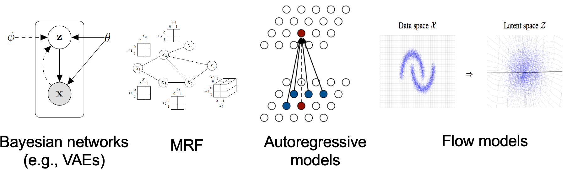
Existing generative modeling techniques can largely be grouped into two categories based on how they represent probability distributions.
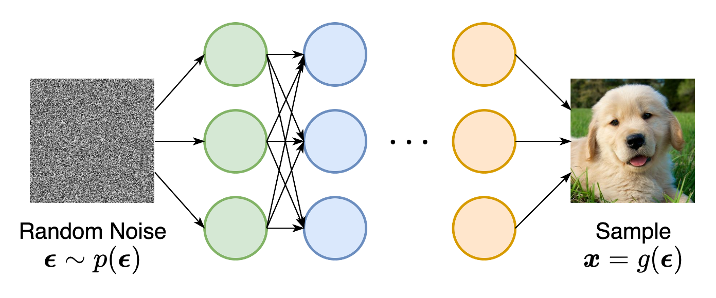
Likelihood-based models and implicit generative models, however, both have significant limitations. Likelihood-based models either require strong restrictions on the model architecture to ensure a tractable normalizing constant for likelihood computation, or must rely on surrogate objectives to approximate maximum likelihood training. Implicit generative models, on the other hand, often require adversarial training, which is notoriously unstable and can lead to mode collapse .
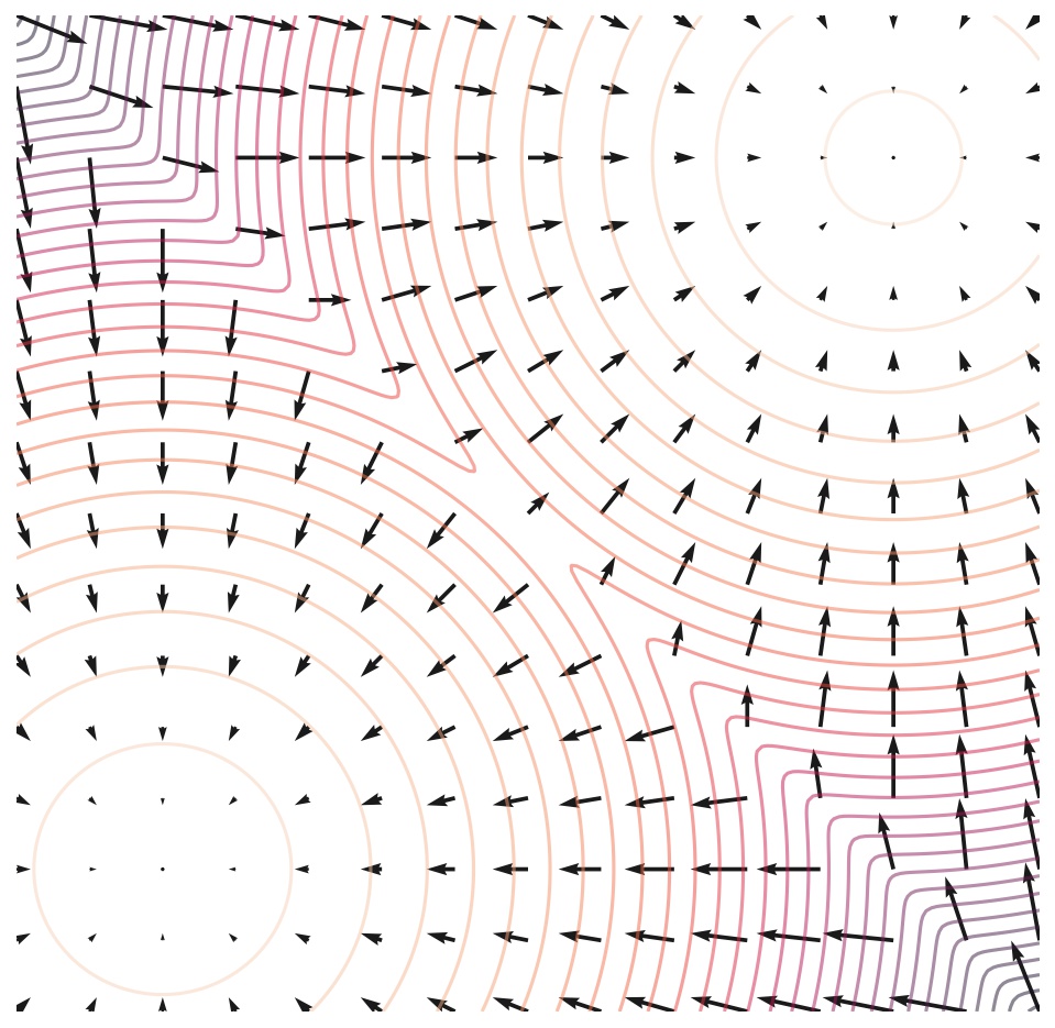
In this blog post, I will introduce another way to represent probability distributions that may circumvent several of these limitations. The key idea is to model the gradient of the log probability density function, a quantity often known as the (Stein) score function . Such score-based models are not required to have a tractable normalizing constant, and can be directly learned by score matching .
Score-based models have achieved state-of-the-art performance on many downstream tasks and applications. These tasks include, among others, image generation (Yes, better than GANs!), audio synthesis , shape generation, and music generation. Moreover, score-based models have connections to normalizing flow models, therefore allowing exact likelihood computation and representation learning. Additionally, modeling and estimating scores facilitates inverse problem solving, with applications such as image inpainting , image colorization , compressive sensing, and medical image reconstruction (e.g., CT, MRI) .

This post aims to show you the motivation and intuition of score-based generative modeling, as well as its basic concepts, properties and applications.
Suppose we are given a dataset \(\{\mathbf{x}_1, \mathbf{x}_2, \cdots, \mathbf{x}_N\}\), where each point is drawn independently from an underlying data distribution \(p(\mathbf{x})\). Given this dataset, the goal of generative modeling is to fit a model to the data distribution such that we can synthesize new data points at will by sampling from the distribution.
In order to build such a generative model, we first need a way to represent a probability distribution. One such way, as in likelihood-based models, is to directly model the probability density function (p.d.f.) or probability mass function (p.m.f.). Let \(f_\theta(\mathbf{x}) \in \mathbb{R}\) be a real-valued function parameterized by a learnable parameter \(\theta\). We can define a p.d.f. Hereafter we only consider probability density functions. Probability mass functions are similar. via \begin{align} p_\theta(\mathbf{x}) = \frac{e^{-f_\theta(\mathbf{x})}}{Z_\theta}, \label{ebm} \end{align} where \(Z_\theta > 0\) is a normalizing constant dependent on \(\theta\), such that \(\int p_\theta(\mathbf{x}) \textrm{d} \mathbf{x} = 1\). Here the function \(f_\theta(\mathbf{x})\) is often called an unnormalized probabilistic model, or energy-based model .
We can train \(p_\theta(\mathbf{x})\) by maximizing the log-likelihood of the data \begin{align} \max_\theta \sum_{i=1}^N \log p_\theta(\mathbf{x}i). \label{mle} \end{align} However, equation \eqref{mle} requires \(p\theta(\mathbf{x})\) to be a normalized probability density function. This is undesirable because in order to compute \(p_\theta(\mathbf{x})\), we must evaluate the normalizing constant \(Z_\theta\)—a typically intractable quantity for any general \(f_\theta(\mathbf{x})\). Thus to make maximum likelihood training feasible, likelihood-based models must either restrict their model architectures (e.g., causal convolutions in autoregressive models, invertible networks in normalizing flow models) to make \(Z_\theta\) tractable, or approximate the normalizing constant (e.g., variational inference in VAEs, or MCMC sampling used in contrastive divergence) which may be computationally expensive.
By modeling the score function instead of the density function, we can sidestep the difficulty of intractable normalizing constants. The score function of a distribution \(p(\mathbf{x})\) is defined as \begin{equation} \nabla_\mathbf{x} \log p(\mathbf{x}), \notag \end{equation} and a model for the score function is called a score-based model , which we denote as \(\mathbf{s}\theta(\mathbf{x})\). The score-based model is learned such that \(\mathbf{s}\theta(\mathbf{x}) \approx \nabla_\mathbf{x} \log p(\mathbf{x})\), and can be parameterized without worrying about the normalizing constant. For example, we can easily parameterize a score-based model with the energy-based model defined in equation \eqref{ebm} , via
\[\begin{equation} \mathbf{s}\theta (\mathbf{x}) = \nabla{\mathbf{x}} \log p_\theta (\mathbf{x} ) = -\nabla_{\mathbf{x}} f_\theta (\mathbf{x}) - \underbrace{\nabla_\mathbf{x} \log Z_\theta}{=0} = -\nabla\mathbf{x} f_\theta(\mathbf{x}). \end{equation}\]
Note that the score-based model \(\mathbf{s}\theta(\mathbf{x})\) is independent of the normalizing constant \(Z\theta\) ! This significantly expands the family of models that we can tractably use, since we don’t need any special architectures to make the normalizing constant tractable.
Similar to likelihood-based models, we can train score-based models by minimizing the Fisher divergence Fisher divergence is typically between two distributions p and q, defined as $$\begin{equation} \mathbb{E}{p(\mathbf{x})}[\| \nabla\mathbf{x} \log p(\mathbf{x}) - \nabla_\mathbf{x}\log q(\mathbf{x}) \|2^2]. \end{equation}$$ Here we slightly abuse the term as the name of a closely related expression for score-based models. between the model and the data distributions, defined as \(\begin{equation} \mathbb{E}{p(\mathbf{x})}[\| \nabla_\mathbf{x} \log p(\mathbf{x}) - \mathbf{s}_\theta(\mathbf{x}) \|_2^2]\label{fisher} \end{equation}\)